An Introduction to Graph Analysis with xGT
Download this jupyter notebook for an interactive experience.
Setting up the xGT environment
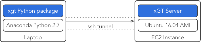
For this demonstration, we'll be running the xGT Server on an Amazon EC2 instance and interacting with it over a secure ssh tunnel from our laptop. More details and alternative methods for getting xGT running can be found at docs.trovares.com.
Install xgt on our local machine
!pip install --quiet --upgrade http://developer.trovares.com/download/python/latest/xgt-latest.tar.gz
Checking the xGT server is up
!ssh cloud ps -e | grep xgtd
1377 ? 00:00:00 xgtd
Establishing a secure tunnel
!ssh -fNL 4367:localhost:4367 ec2-user@cloud
!ps -A | grep 'ssh[ ]-fNL'
44348 ?? 0:00.00 ssh -fNL 4367:localhost:4367 ec2-user@cloud
Getting started with xGT
First, let's import the package and ensure our connection is good.
import xgt
conn = xgt.Connection()
conn
<xgt.connection.Connection at 0x110634390>
Loading data
We'll be using the LANL Unified Host and Network Dataset, a set of netflow and host event data collected on an internal Los Alamos National Lab network.
Our goal will be to turn about 100GB of CSV files into a single connected graph.
Step 1: Create a Graph
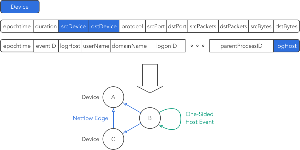
Vertices: Los Alamos uses a free-form, anonymized string called a "device" as a host identifier (analogous to an IP address). We'll use these as vertices in our graph:
[conn.drop_frame(_) for _ in ['Netflow','Events','Devices']]
[True, True, True]
devices = conn.create_vertex_frame(
            name='Devices',
            schema=[['device', xgt.TEXT]],
            key='device')
devices
<xgt.graph.VertexFrame at 0x1042a7110>
Edges: The LANL dataset contains two types of data: netflow and host events. Of the host events recorded, some describe events within a device (e.g., reboots), and some describe events between devices (e.g., login attempts). We'll only be loading the netflow data and in-device events. We call these events "one-sided", since we describe them as graph edges from one vertex to itself.
netflow = conn.create_edge_frame(
            name='Netflow',
            schema=[['epochtime', xgt.INT],
                    ['duration', xgt.INT],
                    ['srcDevice', xgt.TEXT],
                    ['dstDevice', xgt.TEXT],
                    ['protocol', xgt.INT],
                    ['srcPort', xgt.INT],
                    ['dstPort', xgt.INT],
                    ['srcPackets', xgt.INT],
                    ['dstPackets', xgt.INT],
                    ['srcBytes', xgt.INT],
                    ['dstBytes', xgt.INT]],
            source=devices,
            target=devices,
            source_key='srcDevice',
            target_key='dstDevice')
netflow
<xgt.graph.EdgeFrame at 0x10427c4d0>
events = conn.create_edge_frame(
           name='Events',
           schema=[['epochtime', xgt.INT],
                   ['eventID', xgt.INT],
                   ['logHost', xgt.TEXT],
                   ['userName', xgt.TEXT],
                   ['domainName', xgt.TEXT],
                   ['logonID', xgt.INT],
                   ['processName', xgt.TEXT],
                   ['processID', xgt.INT],
                   ['parentProcessName', xgt.TEXT],
                   ['parentProcessID', xgt.INT]],
           source=devices,
           target=devices,
           source_key='logHost',
           target_key='logHost')
events
<xgt.graph.EdgeFrame at 0x104301ed0>
Step 2: Load the data
With all the data types described, we can actually add data fitting those descriptions directly from data files. We load these directly into the edge or vertex structures they correspond to.
# Utility to pretty-print the data currently in xGT
def print_data_summary():
  print('Devices (vertices): {:,}'.format(devices.num_vertices))
  print('Netflow (edges): {:,}'.format(netflow.num_edges))
  print('Host event (edges): {:,}'.format(events.num_edges))

print_data_summary()
Devices (vertices): 0
Netflow (edges): 0
Host event (edges): 0
Load the 1-sided host event data:
%%time
urls = ["http://datasets.trovares.com/LANL/xgt/wls_day-%02d_1v.csv" % int(i) for i in range(4,5)]
#urls = ["xgtd://wls_day-%02d_1v.csv" % int(i) for i in range(4,5)]
events.load(urls)
print_data_summary()
Devices (vertices): 10170
Netflow (edges): 0
Host event (edges): 16402438
CPU times: user 51.2 ms, sys: 15.3 ms, total: 66.5 ms
Wall time: 31.1 s
Load the netflow data:
%%time
urls = ["http://datasets.trovares.com/LANL/xgt/nf_day-%02d.csv" % int(i) for i in range(4,5)]
#urls = ["xgtd://nf_day-%02d.csv" % int(i) for i in range(4,5)]
netflow.load(urls)
print_data_summary()
Devices (vertices): 157949
Netflow (edges): 222323503
Host event (edges): 16402438
CPU times: user 137 ms, sys: 40.8 ms, total: 178 ms
Wall time: 4min 25s
Querying our graph
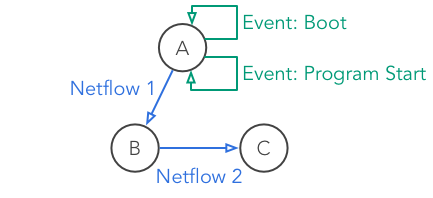
We'll be looking for a mock pattern, similar to one that might be used to detect bot-net behavior. The pattern reflects an infected host (A) which is connecting up to a bot-net command and control node (B) with an exfiltration connection to a collection node (C).
-
Some device A boots up and, within a short amount of time, starts up a program.
-
Shortly afterwards, device A sends a message to some other device B.
-
Device B has a long-standing connection to another device C, which has been open for at least an hour, started before A booted, and remained open after A sent a message to B.
# Query helper function
def run_query_and_count(query):
    conn.drop_frame('answers')
    conn.run_job(query)
    # Retrieve count
    table = conn.get_table_frame('answers')
    count = table.get_data()[0][0]
    return count
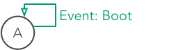
Query 1: Search for just a boot event
Normally, we might not know exactly which pattern to look for, and refining that pattern would be part of the analytic process. We'll start by just finding devices with boot events.
%%time
q = """
MATCH (A)-[boot:Events]->(A)
WHERE boot.eventID = 4608
RETURN COUNT(*)
INTO answers
"""
count = run_query_and_count(q)
print('Number of boot events: ' + '{:,}'.format(count))
Number of boot events: 1,712
CPU times: user 10.9 ms, sys: 4.06 ms, total: 15 ms
Wall time: 446 ms
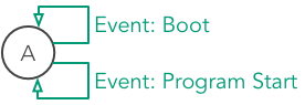
Query 2: Boot event followed by program start event
Now we'll refine the query by looking for programs launched within 4 seconds of a boot event.
%%time
q = """
MATCH (A)-[boot:Events]->(A)-[program:Events]->(A)
WHERE boot.eventID = 4608
  AND program.eventID = 4688
  AND program.epochtime >= boot.epochtime
  AND program.epochtime-boot.epochtime < 4
RETURN COUNT(*)
INTO answers
"""

count = run_query_and_count(q)
print('Number of boot & program start events: ' + '{:,}'.format(count))
Number of boot & program start events: 253,009
CPU times: user 12.8 ms, sys: 4.08 ms, total: 16.8 ms
Wall time: 691 ms
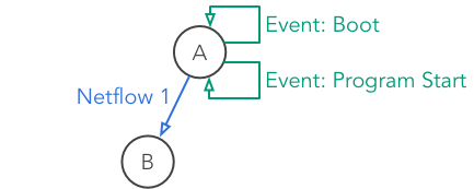
Query 3: Boot, program start, and connection
Now we add the network connection edge from A to B from port 3128 (in our mock example, this is a signature port for the bot in question). We'll restrict it such that all the pieces (boot, program start, and message) happen within 4 seconds.
%%time
q = """
MATCH (B)-[nf1:Netflow]->(A)-[boot:Events]->(A)-[program:Events]->(A)
WHERE A <> B
  AND nf1.srcPort = 3128
  AND boot.eventID = 4608
  AND program.eventID = 4688
  AND program.epochtime >= boot.epochtime
  AND nf1.epochtime >= program.epochtime
  AND nf1.epochtime-boot.epochtime < 4
RETURN COUNT(*)
INTO answers
"""
# Note the overall time limit on the sequence of the three events

count = run_query_and_count(q)
print('Number of boot, programstart, & nf0 events: ' + '{:,}'.format(count))
Number of boot, programstart, & nf0 events: 109
CPU times: user 19.8 ms, sys: 6.28 ms, total: 26.1 ms
Wall time: 3.35 s
Query 4: Full zombie reboot pattern
Finally, we add in the last network connection and match the full pattern.
%%time
q = """
MATCH (B)-[nf1]->(A)-[boot:Events]->(A)-[program:Events]->(A),
      (B)-[nf2]->(C)
WHERE A <> B AND B <> C AND A <> C
  AND nf1.srcPort = 3128
  AND boot.eventID = 4608
  AND program.eventID = 4688
  AND program.epochtime >= boot.epochtime
  AND nf1.epochtime >= program.epochtime
  AND nf1.epochtime-boot.epochtime < 4
  AND nf2.duration >= 3600
  AND nf2.epochtime < nf1.epochtime
  AND nf2.epochtime+nf2.duration >= nf1.epochtime
RETURN COUNT(*)
INTO answers
"""

count = run_query_and_count(q)
print('Number of zombie reboot events: ' + '{:,}'.format(count))
Number of zombie reboot events: 981
CPU times: user 34.2 ms, sys: 10.5 ms, total: 44.8 ms
Wall time: 14.4 s