6.3. Jaccard Similarity
The single-source version of this problem is:
Given a specific vertex A, find other vertices B that are most similar to A.
This is done by computing a similarity metric for each vertex B and then rank-ordering the vertices by that score.
The Jaccard similarity metric is between two different vertices A and B. It is computed as the ratio of the intersection of their neighboring U vertex sets to the union of their neighbor sets. The diagram shows, for a given A and B, a neighborhood union of size 8. The intersection of the two neighborhoods include: {1, 3, 7}, so the intersection size is 3. If the intersection is the same size as the union, that means the two vertices have identical neighborhoods and are therefore considered to be most similar.
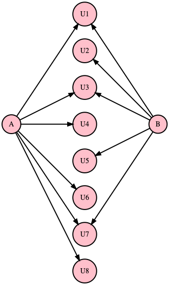
Two Vertices with Similar Neighborhoods
This metric is based on the graph topology and is not influenced by the vertex and edge property values. It may be more interesting to include data values as part of a Jaccard analysis.
The overall flow of this analysis using xGT involves these phases:
Build a connectivity graph to drastically reduce the search space
Compute the Jaccard Scores
6.3.1. Connect to the xGT Server
Before embarking on phase 1, some prelimiaries are required to interact
with the xGT server.
import xgt
import getpass
server=xgt.Connection(auth = xgt.BasicAuth(getpass.getuser(),
                                           getpass.getpass()))
server.server_version
········
'1.8.0'
6.3.2. Retrieve Metadata about the Graph
Select specific parts of the graph to analyze:
A_VERTEX_KEYselects the key of the unique vertex to play the role of A. Note that this vertex is the single source and the Jaccard computation will find other vertices most similar to A.EDGE_FRAME_NAMEis the name of the edge frame connecting A to all of the B vertices.
From the selected information, the components of the graph in the
xGT server are extracted.
A_VERTEX_KEY='VPN'
EDGE_FRAME_NAME='Netflow'

server.set_default_namespace('lanl')

edge = server.get_edge_frame(EDGE_FRAME_NAME)
source_vertex = server.get_vertex_frame(edge.source_name)
target_vertex = server.get_vertex_frame(edge.target_name)
VERTEX_KEY = source_vertex.key

(source_vertex, edge, target_vertex, VERTEX_KEY)
  (<xgt.graph.VertexFrame at 0x111686580>,
   <xgt.graph.EdgeFrame at 0x111686c40>,
   <xgt.graph.VertexFrame at 0x1116868b0>,
   'device')
6.3.3. Define Utility Functions
These utility functions are used during the phases to interact with the
xGT server.
# Utility to print the data sizes currently in xGT
def print_data_summary(server):
    frames = (server.get_table_frames() +
              server.get_vertex_frames() +
              server.get_edge_frames())
    if len(frames)==0:
        print("No data has been defined")
    for frame in frames:
        frame_name = frame.name
        if isinstance(frame, xgt.EdgeFrame):
            frame_type = 'edge'
        elif isinstance(frame, xgt.VertexFrame):
            frame_type = 'vertex'
        elif isinstance(frame, xgt.TableFrame):
            frame_type = 'table'
        else:
            frame_type = 'unknown'
        print("{} ({}): {:,}".format(frame_name, frame_type, frame.num_rows))

print_data_summary(server)
  lanl__Devices (vertex): 157,875
  lanl__Netflow (edge): 222,323,503
6.3.4. Phase 1: Build a Connectivity Graph
Between any two vertices, a -> b, there may be many edges, perhaps
millions.
To compute Jaccard similarity, all we need to know is if there is at least one or if there are zero edges.
We superimpose a connectivity graph on the same vertex set and leave either zero or one edges between every pair of vertices.
This phase consists of finding distinct vertex pairs with at least one edge. Note that this results in a table with the source and target vertex keys. From there we populate a new edge frame.
# create connectivity edge
connected_to_edge = 'ConnectedTo'
server.drop_frame(connected_to_edge)
edge_schema = dict(edge.schema)
connected_to = server.create_edge_frame(
    name=connected_to_edge,
    schema=[[edge.source_key, edge_schema[edge.source_key]],
            [edge.target_key, edge_schema[edge.target_key]]],
    source=edge.source_name,
    target=edge.target_name,
    source_key=edge.source_key,
    target_key=edge.target_key)
connected_to
<xgt.graph.EdgeFrame at 0x111188af0>
%%time
# Find distinct pairs of vertices over edge frame, create one edge for each distinct pair
q = """
MATCH (a)-[e1:{edge_frame}]->(b)
WHERE unique_vertices(a, b)
WITH DISTINCT a, b
CREATE (a)-[e: {connected_to_edge} {{ }}]->(b)
RETURN count(*) AS count
""".format(edge_frame=EDGE_FRAME_NAME,
           connected_to_edge=connected_to_edge
          )
print("query:\n\n{}".format(q))
job = server.run_job(q, parameters={})
print("Number of 'connected_to' edges: {:,}".format(job.get_data()[0][0]))
  query:


  MATCH (a)-[e1:Netflow]->(b)
  WHERE unique_vertices(a, b)
  WITH DISTINCT a, b
  CREATE (a)-[e: ConnectedTo { }]->(b)
  RETURN count(*) AS count

  Number of 'connected_to' edges: 559,680
  CPU times: user 5.85 ms, sys: 6.31 ms, total: 12.2 ms
  Wall time: 9.13 s
6.3.5. Phase 2: Compute the Jaccard scores
This phase finds two-paths from the A vertex to all other B vertices through an intermediate vertex U.
From this information, for each vertex B, the intersection size and union size are computed followed by the ratio (which is the Jaccard score).
We rely on the observation that the outdegree sum is the same as the size of the union of A and B neighborhoods.
We also rely on the observation that the number of two-paths from A to B is the same as the size of the intersection of the two neighborhoods.
%%time
import pandas
q = """
MATCH (a)-[e1:{connected_to_edge}]->(u)<-[e2:{connected_to_edge}]-(b)
WHERE unique_vertices(a, b, u)
  AND a.{vertex_key} = $a_vertex_key
WITH DISTINCT b, u,
     outdegree(a, {connected_to_edge}) + outdegree(b, {connected_to_edge}) AS outDegreeSum
WITH b, outDegreeSum, count(*) AS intersectionSize
WITH b, intersectionSize, outDegreeSum - intersectionSize AS union_size
RETURN
    b.{vertex_key} AS b,
    intersectionSize,
    union_size,
    toFloat(intersectionSize) / union_size AS jaccard_score
ORDER BY jaccard_score DESC
LIMIT 50
""".format(connected_to_edge=connected_to_edge, vertex_key=source_vertex.key)

print("query:\n\n{}".format(q))
job = server.run_job(q, parameters={"a_vertex_key":A_VERTEX_KEY})

df=job.get_data_pandas()
df
  query:


  MATCH (a)-[e1:ConnectedTo]->(u)<-[e2:ConnectedTo]-(b)
  WHERE unique_vertices(a, b, u)
    AND a.device = $a_vertex_key
  WITH DISTINCT b, u,
       outdegree(a, ConnectedTo) + outdegree(b, ConnectedTo) AS outDegreeSum
  WITH b, outDegreeSum, count(*) AS intersectionSize
  WITH b, intersectionSize, outDegreeSum - intersectionSize AS union_size
  RETURN
      b.device AS b,
      intersectionSize,
      union_size,
      toFloat(intersectionSize) / union_size AS jaccard_score
  ORDER BY jaccard_score DESC
  LIMIT 50

  CPU times: user 538 ms, sys: 260 ms, total: 798 ms
  Wall time: 2.8 s
| b | intersectionSize | union_size | jaccard_score | |
|---|---|---|---|---|
| 0 | Comp678443 | 87 | 665 | 0.130827 |
| 1 | Comp030334 | 74 | 781 | 0.094750 |
| 2 | Comp965575 | 72 | 780 | 0.092308 |
| 3 | Comp257274 | 72 | 782 | 0.092072 |
| 4 | Comp866402 | 72 | 783 | 0.091954 |
| 5 | Comp211931 | 50 | 580 | 0.086207 |
| 6 | Comp769797 | 50 | 584 | 0.085616 |
| 7 | Comp148004 | 54 | 637 | 0.084772 |
| 8 | Comp148684 | 49 | 580 | 0.084483 |
| 9 | Comp464369 | 49 | 583 | 0.084048 |
| 10 | Comp889106 | 50 | 598 | 0.083612 |
| 11 | Comp415532 | 48 | 586 | 0.081911 |
| 12 | Comp501848 | 48 | 586 | 0.081911 |
| 13 | Comp725432 | 48 | 592 | 0.081081 |
| 14 | Comp304006 | 47 | 583 | 0.080617 |
| 15 | Comp468329 | 47 | 583 | 0.080617 |
| 16 | Comp055001 | 47 | 585 | 0.080342 |
| 17 | Comp211432 | 46 | 582 | 0.079038 |
| 18 | Comp377866 | 46 | 584 | 0.078767 |
| 19 | Comp507194 | 46 | 584 | 0.078767 |
| 20 | Comp613192 | 46 | 585 | 0.078632 |
| 21 | Comp771132 | 46 | 586 | 0.078498 |
| 22 | Comp599337 | 46 | 587 | 0.078365 |
| 23 | Comp719990 | 45 | 582 | 0.077320 |
| 24 | Comp643534 | 46 | 595 | 0.077311 |
| 25 | Comp881722 | 45 | 583 | 0.077187 |
| 26 | Comp493395 | 45 | 583 | 0.077187 |
| 27 | Comp614801 | 45 | 585 | 0.076923 |
| 28 | Comp764436 | 45 | 586 | 0.076792 |
| 29 | Comp302339 | 45 | 592 | 0.076014 |
| 30 | Comp991220 | 46 | 608 | 0.075658 |
| 31 | Comp130208 | 44 | 582 | 0.075601 |
| 32 | Comp924691 | 45 | 598 | 0.075251 |
| 33 | Comp018032 | 44 | 585 | 0.075214 |
| 34 | Comp943564 | 44 | 585 | 0.075214 |
| 35 | Comp498377 | 44 | 590 | 0.074576 |
| 36 | Comp210768 | 44 | 592 | 0.074324 |
| 37 | Comp688526 | 43 | 581 | 0.074010 |
| 38 | Comp958822 | 43 | 581 | 0.074010 |
| 39 | Comp591316 | 43 | 582 | 0.073883 |
| 40 | Comp856137 | 43 | 582 | 0.073883 |
| 41 | Comp354119 | 43 | 582 | 0.073883 |
| 42 | Comp617264 | 43 | 582 | 0.073883 |
| 43 | Comp498743 | 43 | 583 | 0.073756 |
| 44 | Comp559728 | 43 | 584 | 0.073630 |
| 45 | Comp084630 | 44 | 598 | 0.073579 |
| 46 | Comp356840 | 43 | 585 | 0.073504 |
| 47 | Comp077821 | 43 | 585 | 0.073504 |
| 48 | Comp452053 | 43 | 585 | 0.073504 |
| 49 | Comp959644 | 43 | 587 | 0.073254 |
server.drop_frame(connected_to_edge)
True