2.1. Graph Thinking
2.1.1. Introduction
xGT is a tool for reading in massive amounts of data into RAM for performing fast pattern search operations. The best data for this analytic approach is where there are relationships between data objects described in the data (i.e. linked data). The classic example of this is a social network graph where people have relationships with each other represented in the data such as “friend-of”, “knows”, or “family”.
We start with the assumption you have data and want to analyze it with xGT.
Let’s walk through how to approach this activity, how to build a mental model of your data, how to describe that model using the Rocketgraph xgt Python library, and how to get xGT to help you understand what it is in your data.
After walking through this example, we recommend you review the Jupyter Notebook shown in the Graph Thinking Jupyter Notebook.
We will begin with the data and follow a simple example to illustrate this process. Consider that you have data in two separate comma-separated-values (CSV) files:
Person ID |
Name |
|---|---|
123456789 |
Manny |
123454321 |
Bob |
987654321 |
Frank |
987656789 |
Alice |
Person ID |
Person ID |
Start Date |
End Date |
|---|---|---|---|
123456789 |
987654321 |
2015-01-03 |
2017-04-14 |
123454321 |
987654321 |
2016-04-02 |
2017-04-14 |
987656789 |
987654321 |
2016-07-07 |
2017-04-14 |
123456789 |
987656789 |
2017-04-15 |
|
123454321 |
987656789 |
2017-04-15 |
|
987654321 |
987656789 |
2017-04-15 |
2.1.2. Graph Model
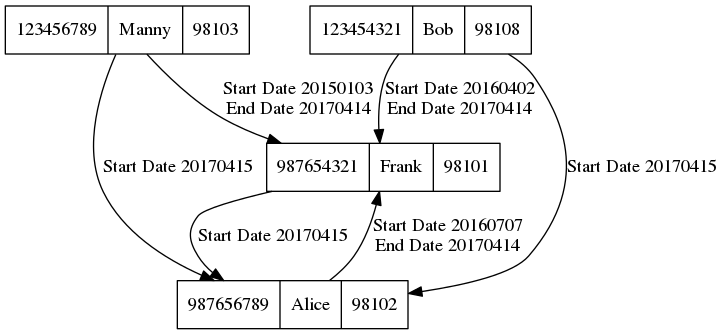
These two data sources correspond nicely to components of a graph. The first is a collection of information about an object (in this case, a person), which can be represented as a vertex in the graph. A vertex is a mathematical name for the “bubble” in a graph drawing.
The second is a collection of information about relationships between objects, which can be represented as an edge in the graph. An edge is a mathematical name for the line that connects two vertices. We usually consider the edge to have a direction, meaning it goes from one specific vertex to another specific vertex. We can call the two vertices in this relationship the source and target of the edge, respectively.
2.1.3. Graph Image
2.1.4. Setting up the Graph Model in xGT 
We can use the xgt library to build a graph model of the CSV data above.
First, we need to describe the kind of data that our graph components will hold.
We create a VertexFrame object which will hold the employee data and an EdgeFrame object which will hold the data describing who reports to whom.
We link vertices and edges by specifying key properties. These relationships give xGT the information required to link this data into a single, connected graph and hop along edges from vertex to vertex quickly and efficiently during queries.
employees = xgt.create_vertex_frame(name   = 'Employees',
                                    schema = [['person_id', xgt.INT],
                                              ['name', xgt.TEXT]],
                                    key    = 'person_id')

reports = xgt.create_edge_frame(name       = 'ReportsTo',
                                schema     = [['employee_id', xgt.INT],
                                              ['boss_id', xgt.INT],
                                              ['start_date', xgt.DATE],
                                              ['end_date', xgt.DATE]],
                                source     = employees,
                                target     = employees,
                                source_key = 'employee_id',
                                target_key = 'boss_id')
2.1.4.1. Understanding the Vertices
As mentioned earlier, the employee data is represented in our graph model as vertices, and each vertex is uniquely identified by a single column from the vertex schema.
All the columns from the vertex schema that are not used as key columns are called properties of the object.
In our case, the vertex frame has a name property for each employee.
2.1.4.2. Understanding the Edges
To connect two vertices (employees) with a ReportsTo relationship we have an edge.
The data associated with each edge comes from the edge’s schema.
Note that there are no columns of the ReportsTo schema that are directly construed as vertices.
The employee_id and boss_id look like identifiers for vertices, but the schema itself doesn’t require that.
Instead, we establish this explicitly using the source, source_key, target, and target_key parameters of the create_edge_frame() method.
The ReportsTo edge connects two Employees vertices therefore the employees vertex frame is used in both source and target parameters of the create_edge_frame() method.
The direction of our ReportsTo relationship is from employee to boss, so the employee_id column is used as the source_key parameter of the edge, and the boss_id column is used as the target_key parameter of the edge.
2.1.4.3. Data Loading
Normally, having described the schema of the graph components, our next step would be to actually fill those components with data from our tables. For brevity, we’ll skip over this step, but you can learn about the various mechanisms xGT provides in our data movement documentation (Data Movement). Let’s pretend we’ve accomplished this and skip straight to searching for patterns in our graph.
2.1.5. Looking for Interesting Patterns
If you have looked over our sample data you may have guessed that one interesting patterns is finding a pattern of an employee (let’s call them “X”) that reports to a boss (“Y”) who later had their roles reversed so “Y” was reporting to “X”.
You can imagine that spotting such a pattern is easy in a few instances, but if you had 100,000 employees to look through, it would be very challenging for a person to notice these kinds of patterns. If your data consisted of employee data from many companies, it is easy to imagine getting to hundreds of millions of graph edges.
So let’s see how to convert our image of a pattern into Rocketgraph’s variant of OpenCypher to have xGT perform an automated search for all patterns.
2.1.5.1. Describing the First Relationship
To describe the first X-Y relationship we formulate a MATCH statement as follows:
MATCH (x:Employees)-[edge1:ReportsTo]->(y:Employees)
Note that all the vertices and edges in the query are annotated with a frame name.
Both vertices are in the Employees frame, and the edge is in the ReportsTo frame.
The xGT data model supports multiple vertex and edge frames in a graph, and xGT must be able to uniquely identify all frames in a query to execute it.
Explicitly annotating all the frames is one way to satisfy this requirement.
But this MATCH statement is incomplete. To finish it, we need to tell xGT what to do with the answers it finds:
MATCH (x:Employees)-[edge1:ReportsTo]->(y:Employees)
RETURN x.person_id, edge1.start_date, edge1.end_date, y.person_id
Be careful: this example produces an exact copy of the ReportsTo table, which may be much larger than you want to deal with.
The original question we asked needs the reverse relationship, too.
2.1.5.2. Describing the Second Relationship
The role-reversing pattern that we want to find can be thought of as a two-path (two contiguous edges) through the graph. At a high level of abstraction, it comes down to: X → Y → X. We also need to add the constraint that the end date of the first edge comes on or before the start date of the second edge.
We begin by showing how to describe a two-path:
MATCH (x:Employees)-[edge1:ReportsTo]->(y)-[edge2]->(x)
RETURN x.person_id, y.person_id,
       edge1.start_date, edge1.end_date,
       edge2.start_date, edge2.end_date
Notice that some frame names were not given in this query. The vertex and edge frame names given are enough to let xGT infer the others.
To add the constraint about the second edge coming on or after the first edge, we add a WHERE clause:
MATCH (x:Employees)-[edge1:ReportsTo]->(y)-[edge2]->(x)
WHERE edge1.end_date <= edge2.start_date
RETURN x.person_id, y.person_id,
       edge1.start_date, edge1.end_date,
       edge2.start_date, edge2.end_date
It is common that queries include constraints in the form of the WHERE clause.
2.1.5.3. Understanding the Query Result
There are really two graphs involved in a query: the large data graph and the smaller query graph. The query graph is the graph structure (vertices and edges) described in the MATCH statement without the constraints of the WHERE clause.
When xGT finds a matching pattern in the large data graph – here “matching” means that the graph structure is aligned and that the attributes attached to the subgraph of the large data graph being matched satisfies the constraints of any WHERE clauses – a row is added to a results table.
The results table will have columns that correspond to the names in the RETURN clause.
If the query has an AS name component in the RETURN clause, name will be used as the name of the column in the results table.
Otherwise, xGT will select a unique name for the results table column.
The data type of each column is automatically determined from the data type of the corresponding return value.
The optional INTO keyword allows specifying a table frame in which to place the results.
If the INTO keyword is not used, the results are placed in the job that ran the query.
MATCH (x:Employees)-[edge1:ReportsTo]->(y)-[edge2]->(x)
WHERE edge1.end_date <= edge2.start_date
RETURN x.person_id AS employee1_id, y.person_id AS employee2_id,
       edge1.start_date AS start1, edge1.end_date AS end1,
       edge2.start_date AS start2, edge2.end_date AS end2
INTO Results
2.1.5.4. Exploring the Query Result
Once a query finishes, xGT will contain a TableFrame that is populated with data that you described in the query.
2.1.6. Concluding Remarks
We’ve presented a mental model of how to work with graphs and graph data and how some snippets of OpenCypher relate to the mental model. To begin working with real data inside xGT, you’re ready to download the xGT Python interface and get started.
There is a simplified version of this example shown in the Quick Start Guide.
A Python-ready example is presented in the next section.
2.1.7. Graph Thinking Jupyter Notebook
You may download this Jupyter Notebook, which supports an interactive environment for the material shown below.
Create these two files and place them on the machine where you are running Jupyter Notebook. The specified file path is relative to the working directory for Jupyter Notebook. Reading from the client filesystem, as is done in this example, is more convenient and is appropriate for small data sizes. However, it is much slower than reading from the server filesystem. For more information, see 2.5 Data Movement.
employees.csv
person_id,name
123456789,Manny
123454321,Bob
987654321,Frank
987656789,Alice
reports.csv
employee_id,boss_id,start_date,end_date
123456789,987654321,2015-01-03,2017-04-14
123454321,987654321,2016-04-02,2017-04-14
987656789,987654321,2016-07-07,2017-04-14
123456789,987656789,2017-04-15,
123454321,987656789,2017-04-15,
987654321,987656789,2017-04-15,
Notice the empty column for end_date in the last three lines. This
results in assigning a NULL value to those properties.
Code to create CSV files
with open('employees.csv', 'w') as emp_file:
    emp_file.write('person_id,name\n')
    emp_file.write('123456789,Manny\n')
    emp_file.write('123454321,Bob\n')
    emp_file.write('987654321,Frank\n')
    emp_file.write('987656789,Alice\n')

with open('reports.csv', 'w') as reports_file:
    reports_file.write('employee_id,boss_id,start_date,end_date\n')
    reports_file.write('123456789,987654321,2015-01-03,2017-04-14\n')
    reports_file.write('123454321,987654321,2016-04-02,2017-04-14\n')
    reports_file.write('987656789,987654321,2016-07-07,2017-04-14\n')
    reports_file.write('123456789,987656789,2017-04-15,\n')
    reports_file.write('123454321,987656789,2017-04-15,\n')
    reports_file.write('987654321,987656789,2017-04-15,\n')
Begin xGT client script
import xgt
# Connect to server
server = xgt.Connection()

# Drop all objects
[server.drop_frame(f) for f in ['ReportsTo', 'Employees']]
# Populate Employee vertices
try:
  employees = server.get_frame('Employees')
except xgt.XgtNameError:
  employees = server.create_vertex_frame(
      name='Employees',
      schema=[['person_id', xgt.INT],
              ['name', xgt.TEXT]],
      key='person_id')

employees.load("employees.csv", header_mode=xgt.HeaderMode.IGNORE)
# Populate Reports edges
try:
  reports = server.get_frame('ReportsTo')
except xgt.XgtNameError:
  reports = server.create_edge_frame(
      name       = 'ReportsTo',
      schema     = [['employee_id', xgt.INT],
                    ['boss_id', xgt.INT],
                    ['start_date', xgt.DATE],
                    ['end_date', xgt.DATE]],
      source     = employees,
      target     = employees,
      source_key = 'employee_id',
      target_key = 'boss_id')

reports.load("reports.csv", header_mode=xgt.HeaderMode.IGNORE)
# Utility to print the data sizes currently in xGT
def print_data_summary(server, frames=None, namespace=None):
    if frames is None:
        frames = server.get_frames()
    for frame in frames:
        frame_name = frame.name
        if namespace is None or frame_name.startswith(namespace):
            if isinstance(frame, xgt.EdgeFrame):
                frame_type = 'edge'
            elif isinstance(frame, xgt.VertexFrame):
                frame_type = 'vertex'
            elif isinstance(frame, xgt.TableFrame):
                frame_type = 'table'
            else:
                frame_type = 'unknown'
            print("{} ({}): {:,}".format(frame_name, frame_type, frame.num_rows))

print_data_summary(server, namespace='example')
# Query in section 4.1.5.1
df = server.run_job("""
    MATCH (x:Employees)-[edge1:ReportsTo]->(y:Employees)
    RETURN x.person_id, edge1.start_date, edge1.end_date, y.person_id
""").get_data(format='pandas')
print("Number of answers: {:,}".format(len(df)))
df
# Query in section 4.1.5.2
df = server.run_job("""
    MATCH (x:Employees)-[edge1:ReportsTo]->(y)-[edge2]->(x)
    WHERE edge1.end_date <= edge2.start_date
    RETURN x.person_id, y.person_id,
           edge1.start_date, edge1.end_date,
           edge2.start_date, edge2.end_date
""").get_data(format='pandas')
print("Number of answers: {:,}".format(len(df)))
df